
Table of Contents
Introduction
How do you determine the shape and strength of all the major reflectors (reflectors are the transitions between rock types) deeper and deeper inside the earth? Reflect sound waves and feed the raw recordings into the world’s best algorithm for unravelling them … This is XWI (the algorithm) created by S-Cube – founded by researchers at Imperial College London.
Think of S-Cube’s avant-garde algorithm – XWI – as the brain behind the earth’s audio. Our human brain processes the sounds that we hear, allowing us to get a coherent signal of the direction that the sound came from, and other information (such as the words that were said). Similarly, this is analogous to the receivers in the earth, which receive a signal and pass it into XWI, which acts like the brain by processing the waves and telling us what is in the subsurface.
XWI does this in a completely unique and innovative way which means that they hold mathematical commercial advantages when pinpointing natural resources deposits (figuring out which reservoirs in the earth have oil and gas), whilst also even storing carbon (underground!) to offset the emissions. The fact that the algorithm can determine which reservoirs are suitable for storing carbon in the subsurface means that we can make the Earth much more clean for the future by reducing emissions.
During my work experience at the company S-Cube, I was set the challenge of working on a highly simplified version of a related problem to which XWI tackles (parameter extraction with 1 unknown instead of several millions in real-life!!), which I found extremely enjoyable solving in Python. My project was titled “Parameter Extraction for 1 unknown”.
In particular, I was exposed to some very important new mathematical concepts, such as the Newton-raphson method, which was thanks to my supervisors: Dr. Nikhil Shah and Dr. John Armitage, who both read Mathematics at Cambridge and Oxford respectively.
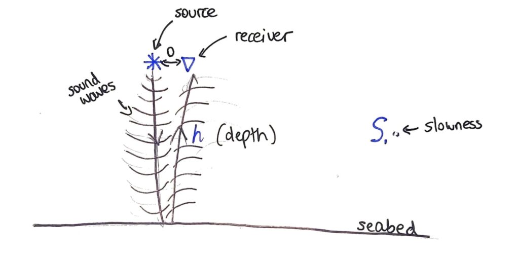
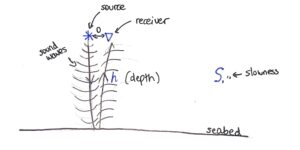
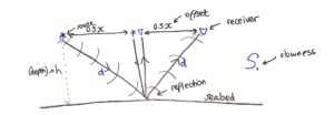
To understand the situation, in Figure 1 below we see that the source sends a sound wave down towards the seabed. Once it hits the seabed, some of the sound waves are reflected back up towards the surface where the receiver receives the waves. (some waves pass through the seabed to the rock layers)
In the first case (Figure 1), the distance between the source and the receiver is set to be 0, so that the depth (h) is simply the vertical distance down to the seabed.
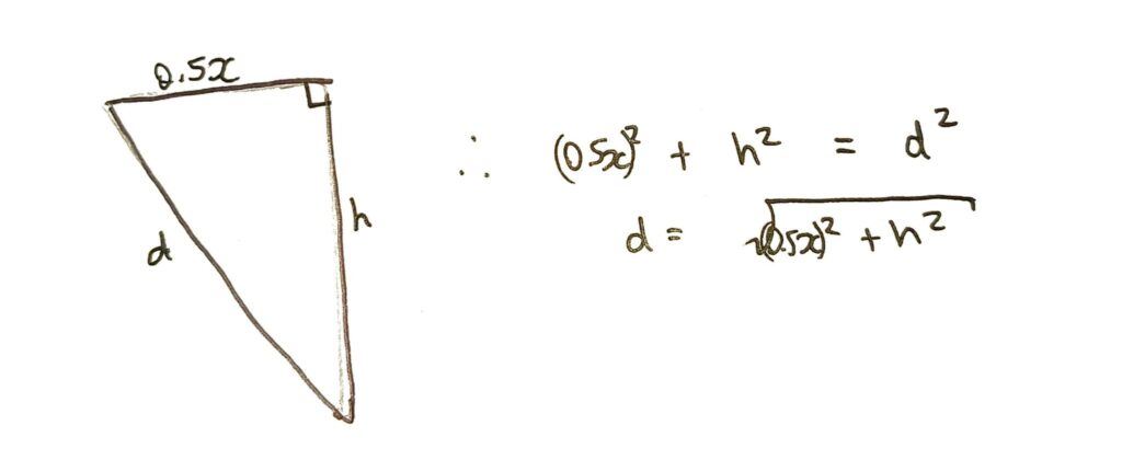
In Figure 2 below, we can setup the source and the receiver at a set distance away from each other, where the offset (x) is the distance from the source in Figure 1 to the source in Figure 2.

Slowness
The term slowness (S1) represents the speed that the wave travels at in the Earth.
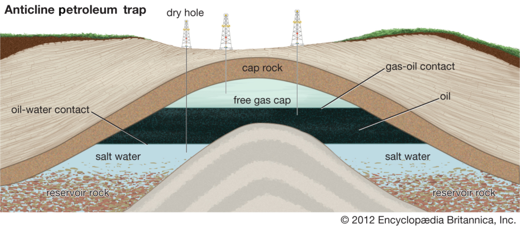
This is a very important parameter to map because slowness shows us all of the geological layers, which form a trap to store a fluid. In Figure 3 below, we can see that high slowness is trapped between low slowness layers – in order to keep the fluid reserves in place (e.g. oil)
If we find out the slowness within a layer, we can tell if that layer contains more fluid (e.g. oil) which is useful to know.
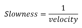
Slowness is the reciprocal of velocity:
Our aim is to find out the travel time for the sound waves from the moment the source sends the wave to the moment the receiver receives the reflected wave.
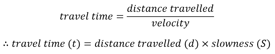
Thus, we can use the following equation to help us work this out. A simple equation is the Time = distance/velocity. Since slowness is the reciprocal of velocity, we have an equation for travel time in terms of distance and slowness.
In this way we can work out the travel time for both Figure 1 and Figure 2, which we will complete below.
Comparison to Image Classification
In order to understand the Parameter extraction task more easily, we will compare the task to image classification in Figure 4 below.
| Parameter extraction (inversion) | Image Classification | |
| Model | slowness, reflector (h) | Neural network |
| True data | travel times | What the images are of |
| Input | pulse (from the loudspeaker) | Images |
| Predicted Data | model travel times | What the neural network thinks the images are of |
| Updated model | change slowness | Update classification of image |
| AIM | To find the values of the true model (hidden slowness value) | Classify image correctly |
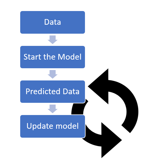
Overview of the model
The simple diagram of how the program will work is in Figure 5. We define the true data (which is hidden to the program, as this is what we are trying to find).
Next we start our model with a guess input, which outputs predicted data. We calculate the error (misfit) between our predicted data and the original true data, and then update the model accordingly.
These last 2 steps are looped until the predicted data is as close as it can be to the original true data.
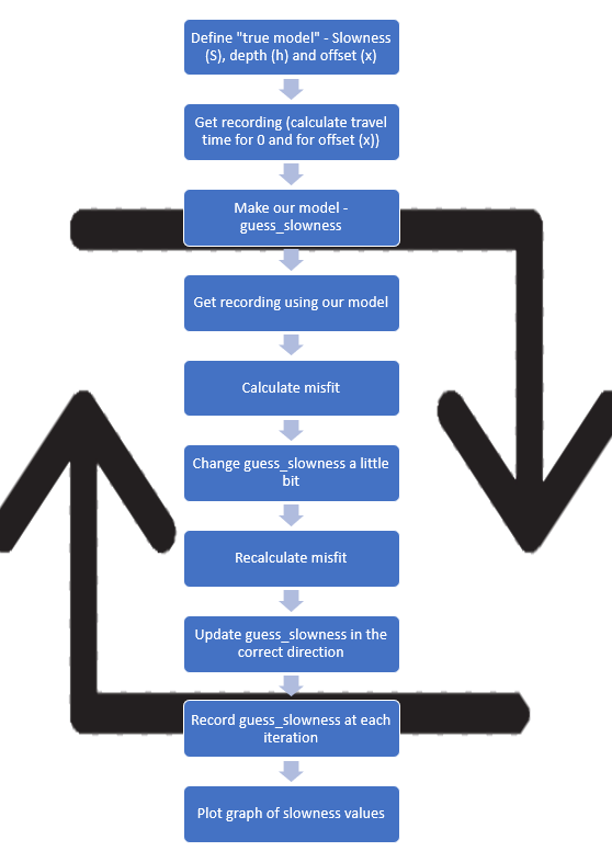
Overview of our Parameter Extraction problem
Figure 6 shows the overview of the steps taken by the program to complete the Parameter extraction problem. I will go into more detail for each step below.
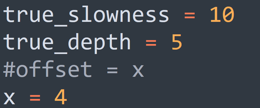
Define True Model
In our example, the true original data is simply the observed data from a “real-world” seabed. We can work out the depth, and the slowness values – and store this into our program. (this data is ‘hidden’ because using our model we want to get closer and closer to this value from a random guess input value for the slowness). Figure 7 shows us define this true data:
Calculate recording (for travel time)
The next step involves taking the true model that we defined above and working out the True travel times (t twiddle/tilde) for the model.
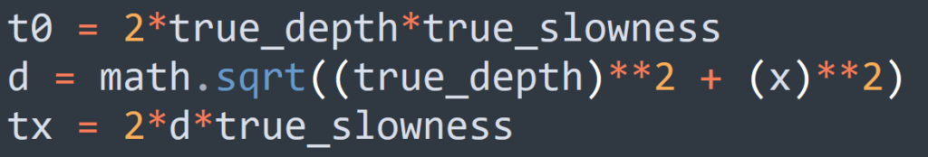
In order to work out the travel time for the diagram in Figure 1 (where distance between source and receiver was 0), we use the equation below. The true_depth (h) multiplied by 2 because the total distance travelled by the sound wave is down to the seabed and back up again from the seabed.

Now that we have the distance travelled (2d), we can use the following equation to work out the travel time for (t twiddle x):

The code for the steps stated above is shown in Figure 9. In order to use the “math.sqrt” function, we had to import the math library at the start of our function.
Make our starting model
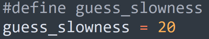
Now that the true model has been defined, we make our model by firstly defining guess_slowness, which is what our model will start with. The aim of the model is to keep looping around the model in order to get this guess_slowness value as close as possible to the true_slowness value defined above.
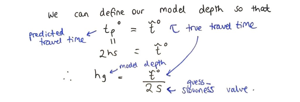
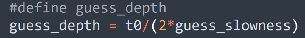
Defining our model depth (see Figure 11), and the code for it in Figure 12.
Calculate recording (for travel time) using our Model
Now that we use got our guess_slowness and guess_depth values, we need to calculate the travel time using these values, similar to the steps in Figure 9.
In Figure 13, “tpx” simply means the predicted travel time value for the x-offset value. “d_guess” is now our guess distance value using our guess_depth value which we defined above.

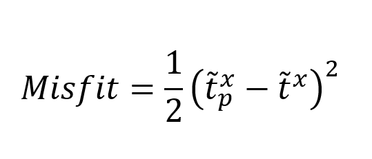
Calculate Misfit
A misfit function simply measures how closely our model’s predicted values are to the true values.
The formula for misfit is shown in Figure 14. Simply put, we are comparing our “tpx” value (predicted travel time) which we calculated in Figure 13 to the “t twiddle x” value (true value) which we defined in Figure 9. This will tell us how much error we have created compared to the true value.

Change guess_slowness value
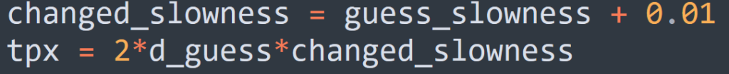
After calculating this misfit, we can now change our guess_slowness value by a small amount (10^-2) – and then see what effect that has on the misfit. The code in Figure 15 shows how adding 0.01 to the previous guess_slowness value, and then we recalculate our travel time value.
Recalculate Misfit and Compare
After changing our predicted travel time value, we can now recalculate our misfit to see whether the change we made was beneficial or not.

Figure 16 shows the code used to compare the two misfit values.
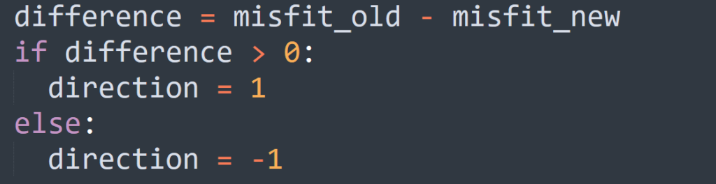
If the difference between the old and new misfit value is greater than 0, it means that the misfit_new is smaller and the smaller the misfit, the more accurate the slowness value, because it is closer to the true slowness value. This means that the direction we want to go is positive (we can keep adding 0.01 to the guess_slowness value until we get close to the true value).
See Figure 17 to see how we must travel in the direction which will take the graph to y = 0.
If the difference between the old and new misfit is less than 0, it means that the misfit_new is larger than the misfit_old, which means we are going in the wrong direction, because we are getting further away from the true value of the slowness. This means that direction = -1, so that the program knows that we need to subtract 0.01 each time to get closer to the true value.

Update guess_slowness in the correct direction
Now that we have worked out the direction in which we want to go, we can simply update the direction in which we change guess_slowness each iteration.
Figure 18 shows the code which we use to update the direction.

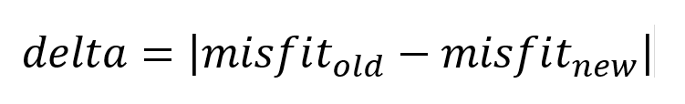
Delta stores the absolute value of the difference between misfit_old and misfit_new:
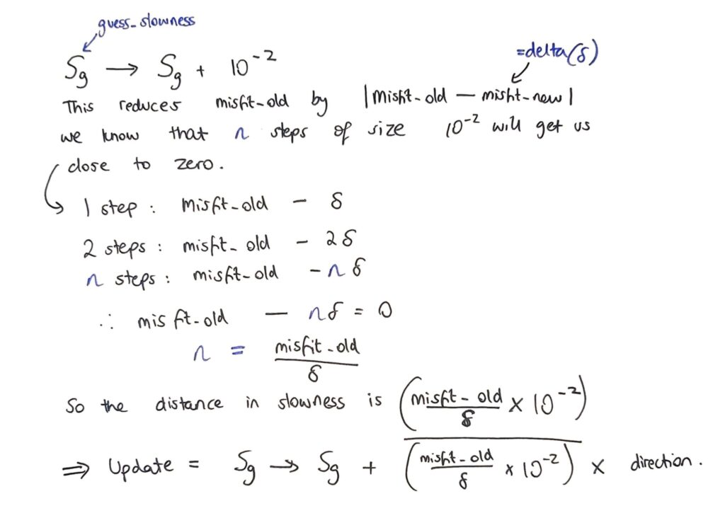
To find out what we need to update, we can follow the steps shown in Figure 19:
Record guess_slowness in each iteration
As shown in Figure 6, there is a loop in our program. This loop will keep updating our model and checking that the misfit is getting smaller and smaller. Just for the purpose of the project, the loop I made will iterate through 10 times:

At the bottom of the loop (before iterating again), the new guess_slowness value is appended to an array called slowness_array. This is so that we can plot the graph in the next step.

Plot graph of guess_slowness values
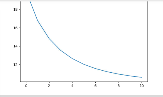
Finally, to show our model working in action, we want to display a graph to show our guess_slowness values getting closer and closer to the true value (where y = 0 is the ideal!).
To plot a graph we import another library called matplotlib at the start of our code, and then we can use the code in Figure 20 to plot the graph:

The graph that we get from our code is shown in Figure 21, which shows that over our 10 iterations, the value for guess_slowness gets more accurate each time – due to our calculations using the misfit values.
The Newton-Raphson Method (Newton’s method)
Our project above finds the minimum of f(x) in order to get an accurate answer for the guess_slowness value.
The Newton-Raphson method is an algorithm used to efficiently and quickly produce successively better approximations to the roots of a real-valued function. The method involves using straight-line tangents to find the approximations of the result.
Essentially, a summary is finding x such that f(x) = 0.
How does the method work? Visual representation:
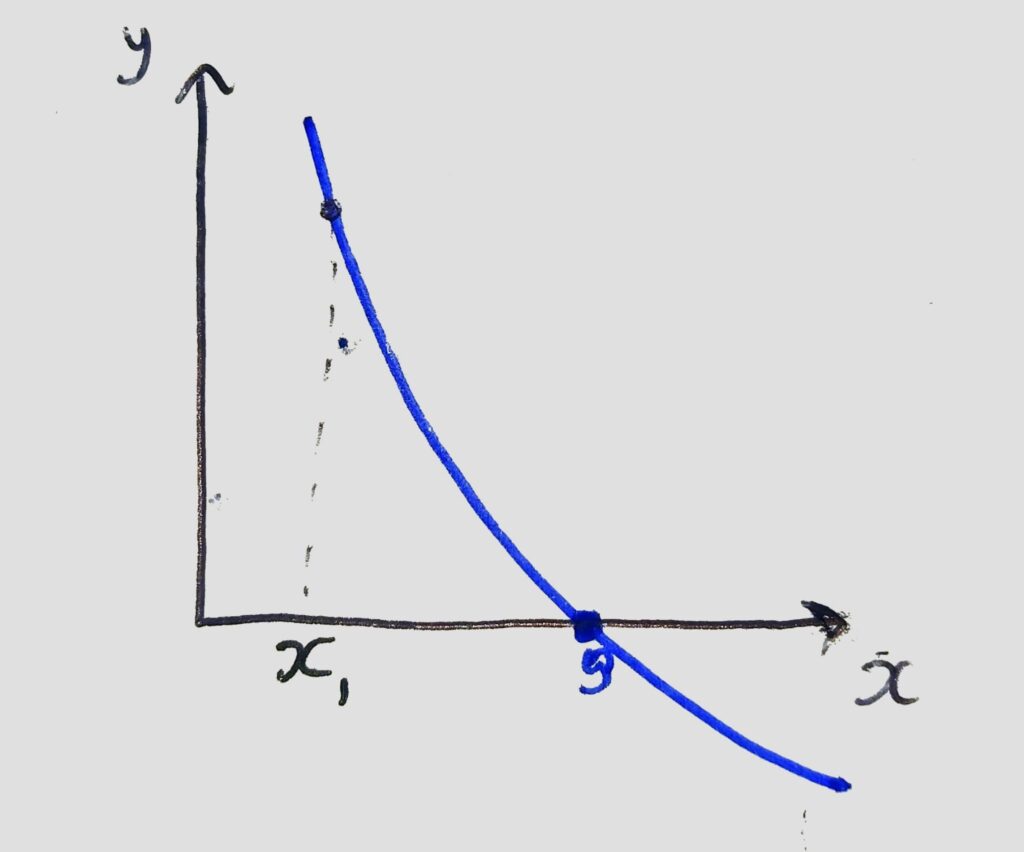
The end goal is to find the point where f(x) = 0 – i.e. the point marked g in Figure 22.

To start with, we make an initial guess called x1. We calculate f(x1) and the most likely case is that f(x1) is not equal to 0 (if it is… then we are very lucky and our job is complete). This is show in Figure 23.
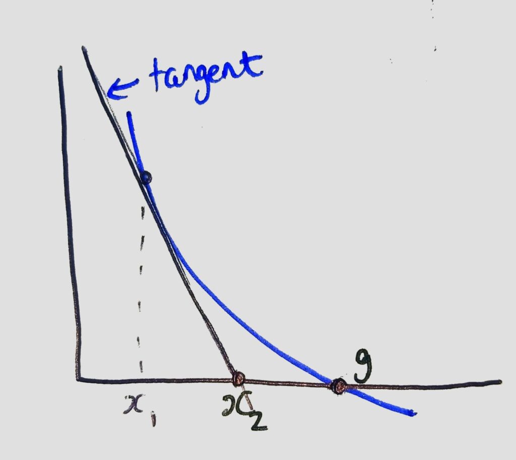
Now that we have tried x1, we now want to try again with a better guess. Newton’s method says that we should draw a tangent to the graph at the point (x1, f(x1)) for a good linear approximation, and where this tangent crosses the x-axis is our x2 – our next guess. See Figure 24.
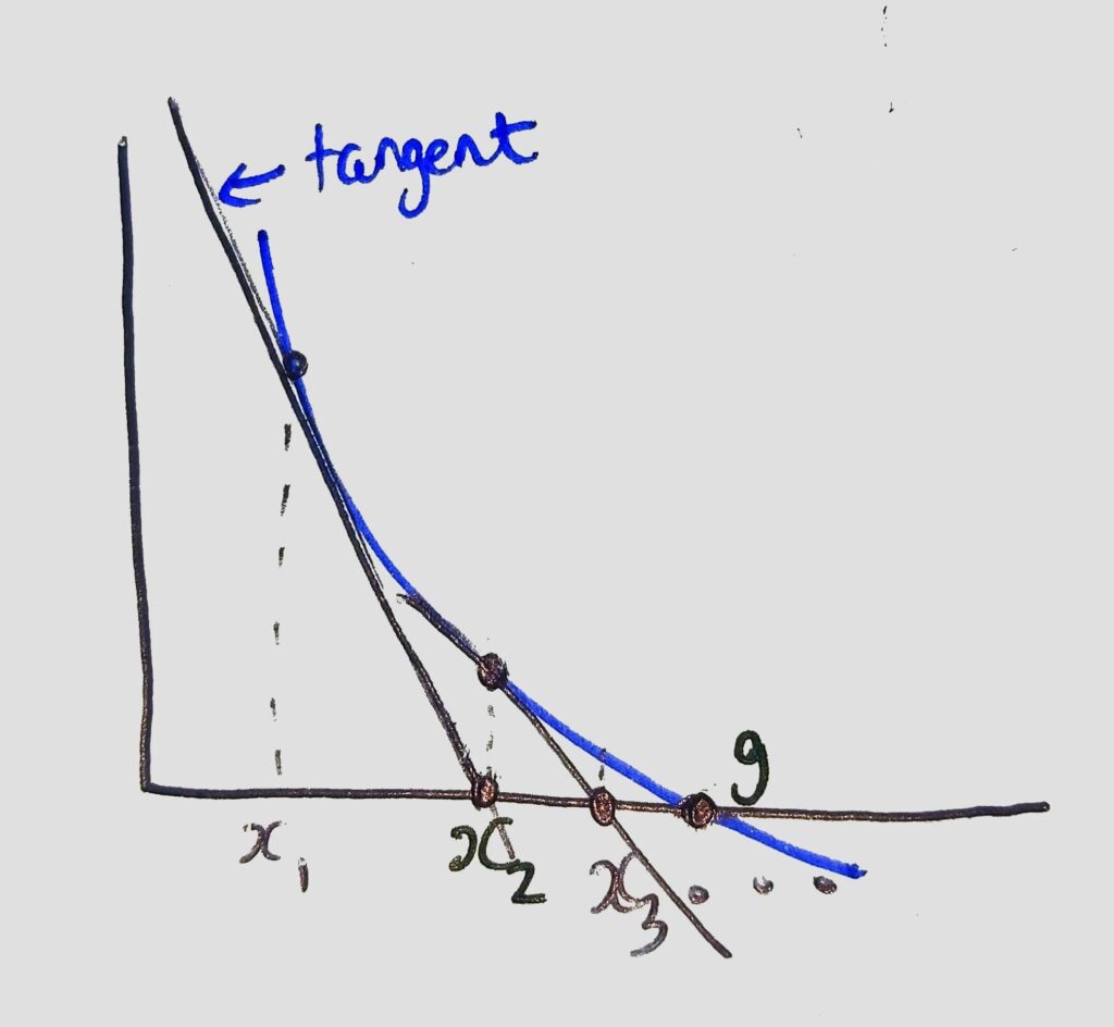
Essentially, this process is continued for x3, x4, x5 … until we hit point g, where f(x) = 0. In figure 25, you can see that with this method, we are quickly getting closer and closer to the root of f(x).
How does the method work? Mathematical representation:
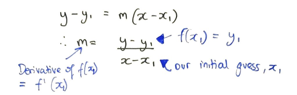
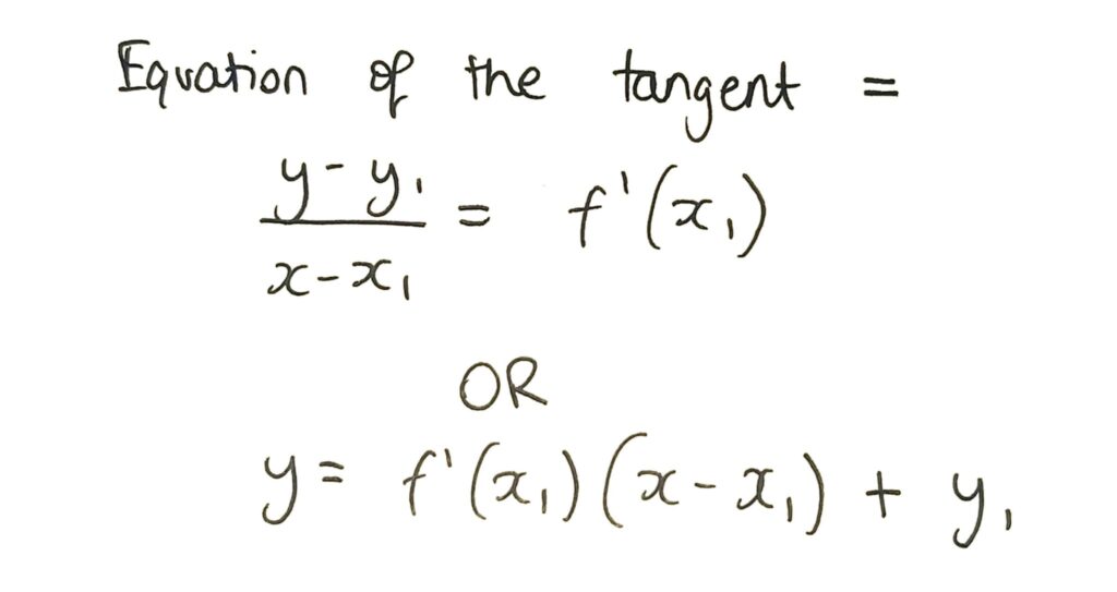
The most important step in Newton’s method is to find where the tangent to x1 meets the x-axis, because this gives us our next better guess.
We need to find this x-intercept, and thus we need to find the equation of the tangent line. Figure 26 and 27 show how we can find the equation of the tangent using the equation of a line.
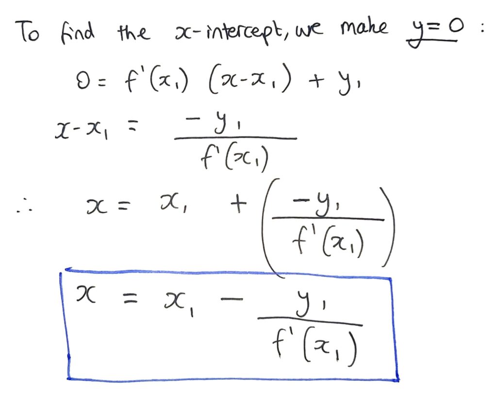
Thus, we can now find the x-intercept of the tangent, as shown in Figure 28:
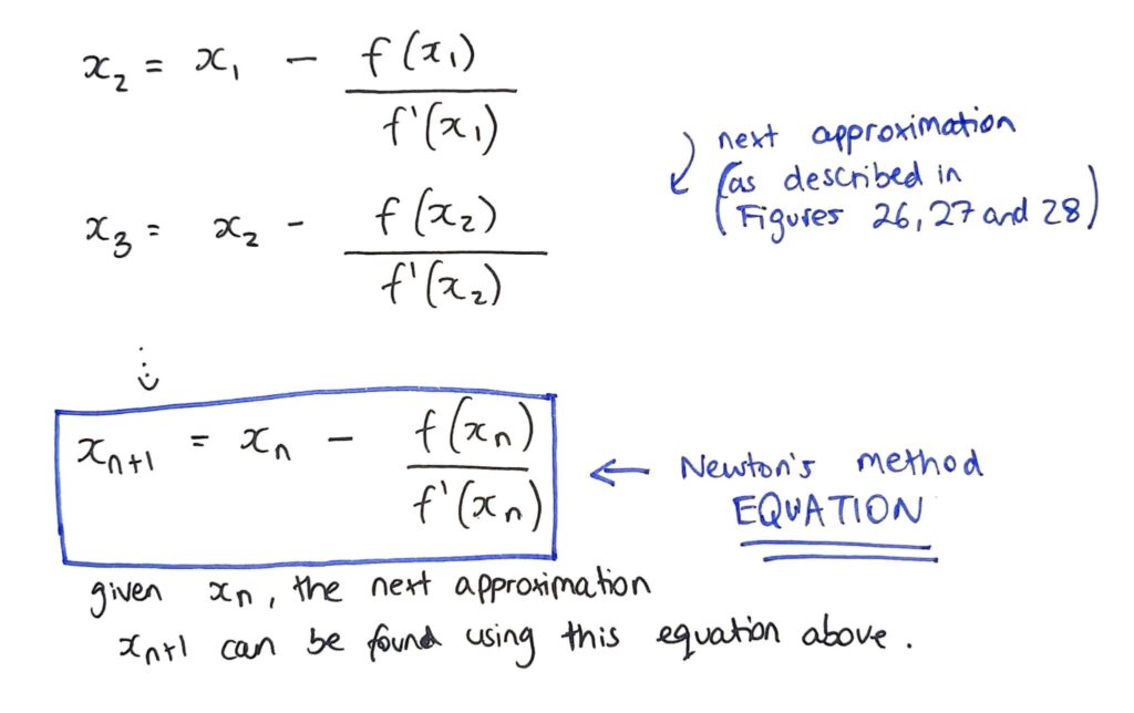
Newton’s method Equation
Therefore, by following the exact same method – we can now show the equation of Newton’s method algebraically, as shown in Figure 29.
Conclusion
This project would not have been possible without the kind support, encouragement and explanations by the team at S-Cube, specifically Dr. Nikhil Shah and Dr. John Armitage. Thank you very much for your time and guidance. I learn several new skills and topics, as well as learning how to link mathematics to real-world solutions, such as S-Cube’s award-winning XWI waveform algorithm.
My project now is to solve the same parameter extraction problem, but instead for multiple layers where slowness and depth are unknown (instead of just slowness).This is a more realistic scenario in real-world earth surveying, because there are multiple unknowns to solve for.
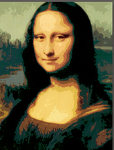
For example, in the Mona Lisa image below, there are millions of pixels, where each pixel is an unknown to be found. It requires a very complex algorithm and powerful computer to solve for one million unknown simultaneously!
I hope you enjoyed reading this article – please feel free to leave any comments/feedback below (in the comments box). Thank you!