
Contents:
- Introduction to the Project
- What is a muon?
- Using Python
- Curve-Fitting
- Residual plots
- Peak-Finding algorithm
- MuSpinSim Simulation
- Docstrings
- Overview
Over 12th – 16th July 2021, I was fortunate to be able to gain a spectacular experience at The Science and Technology Facilities Council (STFC) – albeit virtually. The STFC is one of Europe’s largest research organisations, which assists scientists, engineers and researchers to run experiments around the world. Some of the most interesting topics include particle physics, space exploration, accelerator-based technologies and computer science!
I was a part of the Scientific Computing department at STFC, where I was participating in an intensive one-week virtual project placement. My project was titled:
“Using simulations of muon experiments to aid in analysis and understanding of experimental data for both known and unknown samples”
Introduction to the Project
This project was based upon the fundamental ideas of MUONS, which are simply ‘heavy’ versions of electrons that only live for 2 millionths of a second. (read more about What muons are below…)
Scientists make these muons, and then fire them into materials that we want to study. This is because the muons will mingle among the atoms deep inside of the material, and eventually, they will help us understand what the atoms are doing.
My project was focussed upon an experimental technique called muon SPECTROSCOPY, which is when scientists track the decay of muons into positrons. This allows us to obtain a very detailed image of the magnetic structure of small-scale samples.
The current situation is that muon spectroscopy experiments are expensive, because they require specialised machines and multiple teams of scientists to operate them. And thus, scientists have to apply for “beam time” many months in advance.
Our aim was to write a computer model that can simulate the muon beam and the target material, so that we can simulate all the experiments that we want on the servers that STFC own. These simulations are vital in allowing scientists to understand and analyse unknown samples, as well as find relationships between input conditions and outputs.
What is a ‘muon‘ and what is ‘muon spectroscopy‘?
Muons are simply ‘heavier’ electrons, that only live for 2 millionths of a second. In this way, the muons are unstable (do not exist for long), which means that they drop to a lower energy state, which involves decaying into positrons and other smaller particles.
These positrons are vital in helping us learn more about the muon. The majority of these positrons move along in the direction in which the muons were spinning in when they decayed. Thus, if we collect the positrons, and find which direction they move in, we can find the direction in which the muons were spinning in before they decayed. This helps us build up a picture of what the muons were doing and why they decayed inn a specific direction.
The end goal of our project was to use the real detector data from an unknown magnetic sample (experiment conducted in Canada 🇨🇦) – analyse it and then extract the key information from it.
We can use this extracted information as an input to our simulation (MuSpinSim) – and then try and match the simulation data to the experimental data. If the data matches, then we have found out the input conditions that may have been the possible ones of the original, unknown sample.

Using Python to help with the Simulation:
The programming language that we used to help run our simulation was PYTHON – one of the most widely used languages in the world. I was interested to learn that my supervisor (Josh) uses Python as his primary programming language in the Scientific Computing department!
Firstly, I had to plot the experimental data from the CSV (Excel) file using Python, which meant that I had to setup a Python environment with the following libraries: numpy, scipy, matplotlib etc. because they would help me use scientific python functions.
Having created a function called “import_excel_file”, I used the following line of code to read the CSV file:
np.genfromtext # this is handled by numpy (np) From the CSV file, the original data was read in as a series of [x,y] coordinate pairs. However, we wanted the data as x-values and y-values in 2 separate arrays, which is why we used the line of code with the .T in it, which transposes the data.
data = data[1:].T # .T = transposing the data After completing the rest of the code, I managed to plot and display the data included in the CSV file, which was the basis of the entire project.
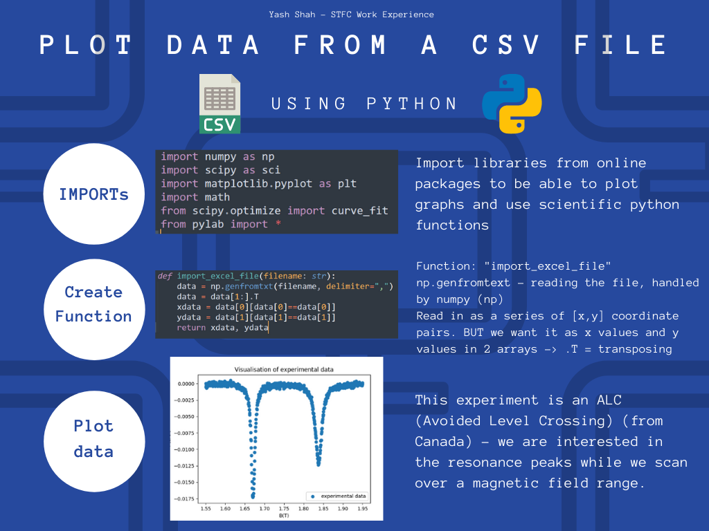
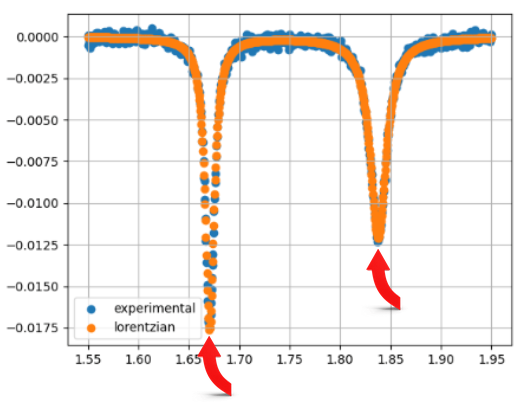
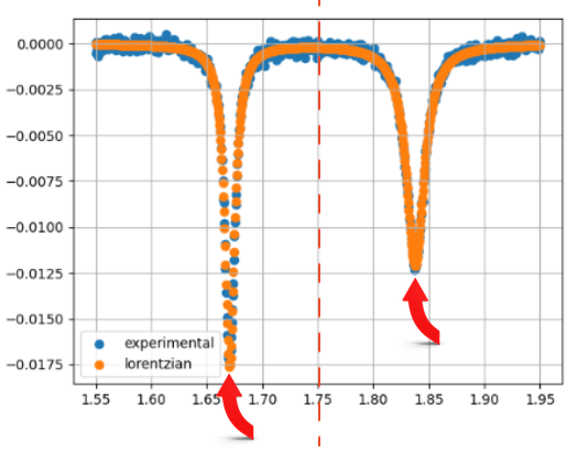
In the graph above, the resonance peaks are the 2 lowest points on the graph – with x-values of approximately 1.66 and 1.84. The data from the positrons gives us these resonance peaks of the muons, which is when the muons give a stronger emission in one direction (due to the movement of the positrons). With these peaks, we can work out the frequency, which is an input into the simulation we used – MuSpinSim.
Curve-Fitting
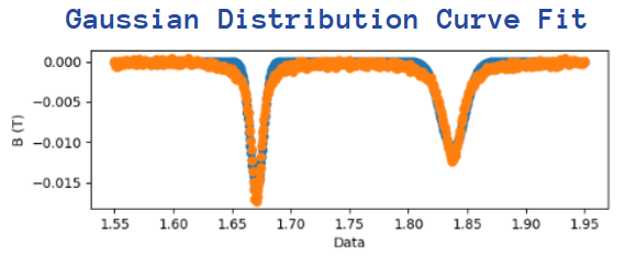
After plotting the experimental data from the original CSV file, my aim was to now perform a curve-fit onto the graph. This is so that we can try and re-create the same curve using Functions we already know about, such as Gaussian or Lorentzian functions. In this way, if our curve-fit matches the original graph, we can learn more about the unknown sample from the experiment.
Gaussian Function
The first function I used was a Gaussian function – which is a normal distribution graph, with a bell-shaped curve.

The following line of code is the equation being put into a line of code:
return -np.exp(-0.5*(((x-mean)/width)**2))/(width*np.sqrt(2*np.pi)) * AThe image below shows the Gaussian Distribution curve-fit (orange curve) on top of the experimental data (blue curve). Although most of the orange curve is matching the blue curve, we can see that the corners of the graph are not a great fit which means that this function is not the perfect curve-fit.
Residual Plots
Before moving onto the second distribution function, an important graph that I used was a residual plot graph.
The residual is the difference between the simulated Y-value and the experimental Y-value
Simply put, the residual shows the difference between the curve-fit data and the original experimental data at every index. This is important because it gives us a clear indication as to how good our curve-fit is.
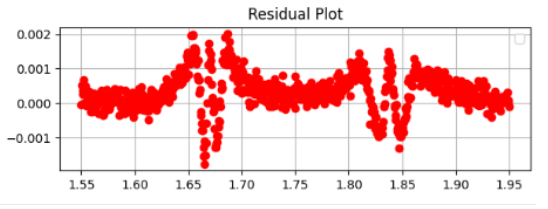
Thus, for the Gaussian distribution graph, the residual plot (red dots) shows that there is a fairly large error between our curve fit and the experimental data. This is because the dots are spread out along the graph are are not in a flat line.
The flatter the residual plot, the lower the error and therefore the better the fit
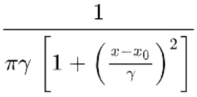
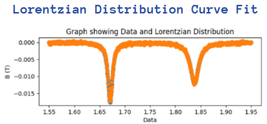
Lorentzian Function
Unlike the Gaussian function, the Lorentzian function has a different mathematical equation: (where γ is the scaling factor, and x0 is the mean)
Similarly, I put the following equation into Python code, so that the program can understand how to plot the graph:
After plotting this new curve-fit on top of our experimental data, the following image shows that the Lorentzian function gives us a smooth and better fit (simply because we can barely see the blue curve from the experimental data). The corners are much sharper compared to the Gaussian function and the orange curve fits exactly on top of the blue curve.
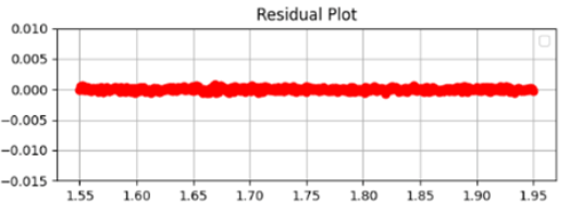
Hence, the residual plot of the Lorentzian function is also much better, because we get a nearly flat red line on the residual plot, showing how perfect the fit is because there is very little difference between the simulated Y-values and the experimental Y-values of the graph.
Peak-finding algorithm
Having completed the two curve-fits, my next task was to make an algorithm to automatically locate the two resonance peaks of the graph.
An algorithm is a procedure or formula for solving a problem, by running a sequence of specified code
For our previous graphs, we gave the program an initial guess as to where the peak might be. But to make the program more efficient, we want the algorithm to find this for us…
The reason we are giving our program these guesses is to do with Big-O notation, which is when we quantify how long a program will take to run. The time it takes for our simulation to find an optimal solution for the graph scales with n^2, where n is the number of parameters (inputs into our function).
This means that if the algorithm already knows 2 accurate peaks, we have eliminated 2 parameters, which means that the time taken to find the optimal solution is reduced, which ultimately saves money (due to the cost of running the servers).
So how do we go about finding the peaks automatically?
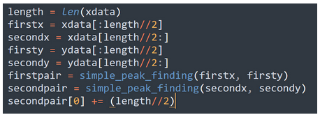
Our algorithm slices the data set into 2 parts, and then finds the minimum point of each half. This is because the minimum point of each side of the graph will be the lowest Y-value, i.e. the peak. Finally, our algorithm returns the x-value of the the minimum point.
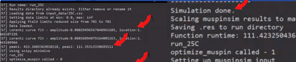
MuSpinSim Simulation
In order to use all the code we had put together, and learn more about the original muons, we used a simulation called MuSpinSim.
There are 3 terms that I will define before explaining how to find out our result to the simulation:
SCARF is the computer cluster that we run the code on (belongs to the STFC)
SLURM is the batch management system on the computer cluster, which decides the order in which tasks should be run
BASH is the scripting language which is used to automate the submission of our jobs
From the previous peak-finding algorithm, we now have the resonance peaks for the experimental graph. This means that we know something is happening in the sample at those specific magnetic fields (the x-values of the minimum points).
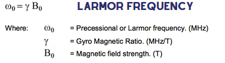
We can convert these magnetic field values (x-values of the minimum points) to frequency using an equation called Larmor frequency:
If we use this frequency as an input to the simulation MuSpinSim, then it calculates another term called the hyperfine coupling term, which is the term that determines the output of MuSpinSim. If our output graph matches the original experimental graph, we can say that the hyperfine coupling term that we have calculated is probably the same as the original experiment. Essentially, this is the ideal result that we are trying to work out from our program.
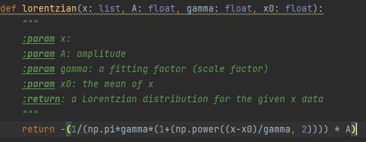
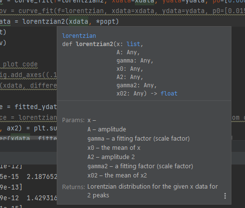
Docstrings
During the work experience, I was taught how to make a docstring (short for Python documentation) for a function that I had written. A docstring is very useful for other programmers to use your function again, because it gives them information about the parameters of the function (i.e. what needs to be inputted into the function and the data type that these variables take). Also, it gives information as to what is returned from the function.
An example of my docstring is shown below, for the function “lorentzian2”. Under the heading “Params:” we see the input parameters to the function, and under “Returns” we see what will be returned from this function, which is the Lorentzian distribution graph.
I learnt that documenting code is very important; not only for others to read and understand the code, but also for yourself. When working on a large code base, it is possible to forget the purpose of previous functions, as well as its inputs and outputs.
Overview
It is interesting to note that the project which I was working on is an area of active research, which many scientists are focussing on.
This work experience was an immensely valuable opportunity where I developed my Python skills such as creating my own modules; my Physics knowledge on muon spectroscopy, as well as my problem-solving skills (we spent 2 hours one evening on a simple problem!) My presentation and communication skills were most definitely developed because I presented my project to all of the people involved in the work experience at the end of the week.
These are all transferable skills that I will be able to use in every aspect of my future career, such as during my A-Levels and higher education.
My greatest achievement from this work experience was that the peak-finding algorithm which I coded will be used in the real code base for the STFC’s Scientific Computing department.
If I had another 2 weeks, I would have liked to experiment with a a few more simulations and learn more of the physics behind this powerful simulation.
I would like to specifically thank Josh Owen, my fantastic supervisor, for all of his support and encourgament when helping me understand this project. Thank you to Lauren and Gemma for organising the work experience, and to STFC for giving me this opportunity to develop many skills during the Summer holidays.
Josh Owen’s reference:

Yash completed a week long work experience placement with myself and the Theoretical and Computational Physics Group at STFC in July 2021. During the course of this, he was engaged and proactive in the work, asking relevant questions and ensuring that he understood both the goals for the week, and the motivation behind the work and its applications to STFCs wider work and research.
Through a mix of independent work, and collaborative problem solving, Yash was able to familiarise himself with part of the existing codebase, identify an improvement in a data fitting technique, and implement his changes successfully. Further, he presented his work to an audience of peers and staff at STFC in a clear and concise manner at the end of the week. I was particularly impressed at the end of his presentation where he demonstrated that was able to explain in detail the motivations for how and why certain decisions were made when asked about this during the questions session.
Overall, Yash was enthusiastic in his work, confident in asking questions to ensure he understood the tasks at hand, and able to perform technical work independently and collaboratively.
Josh Owen
Supervisor: Scientific Computing Department (STFC)